How Neural Networks Learn (Forward & Backward Propagation)

Hey folks,

Last week we covered the building blocks of neural networks - neurons, weights, and biases. Today we're diving into the magic part: how neural networks actually learn.

Remember the formula we showed you last time?

Output = (Input1 × Weight1) + (Input2 × Weight2) + ... + Bias
Final Output = Activation Function (Output)

That's a single neuron. Now, what happens when you stack many neurons in many layers? How does data flow through all of them? And how does the network learn which weights are correct?

Let's break it down.

How Data Flows Through the Network (Forward Propagation)

When you feed data into a neural network, something happens step by step.

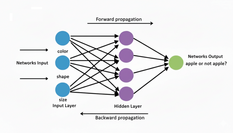
Let me use a simple example. Imagine we have a network to identify if something is an apple or not.

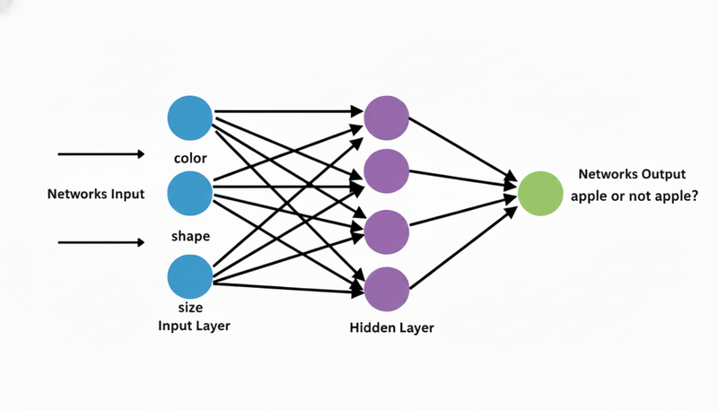
• Input layer: 3 neurons (color, shape, size features)
• Hidden layer: 4 neurons (learning to recognize patterns)
• Output layer: 1 neuron (apple or not apple? 0 to 1)

Here's what happens:

Input Layer

Data comes in. Let's say we're analyzing an image and it gives us:

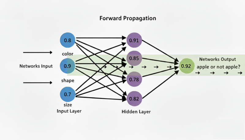
Input = [0.8, 0.9, 0.7]

Hidden Layer

Each neuron in the hidden layer takes ALL inputs and does the calculation:

For neuron 1 in hidden layer:

Output = (0.8 × w1) + (0.9 × w2) + (0.7 × w3) + bias
Output = (0.8 × 0.5) + (0.9 × 0.3) + (0.7 × 0.2) + 0.1
Output = 0.4 + 0.27 + 0.14 + 0.1 = 0.91
After activation: 0.91

For neurons 2, 3, and 4 in the hidden layer, the same process repeats with different weights.

Output Layer

Now the 4 outputs from the hidden layer become inputs to the output layer. Same process repeats:

Output = (h1 × w1) + (h2 × w2) + (h3 × w3) + (h4 × w4) + bias

Where h1, h2, h3, h4 are the 4 values coming from the hidden layer neurons.

Finally, we get our prediction:

Output = 0.92 (92% sure it's an apple)

This entire process - data flowing from input layer → hidden layers → output layer - is called Forward Propagation. We move forward through the network, calculating values at each neuron.

Why do we call it forward propagation?

• We start at the beginning (input)
• We move forward through each layer
• We end at the output
• Each layer's output becomes the next layer's input

The Problem - Our First Prediction is Wrong!

Here's the thing: when the network first starts, the weights are random. So our prediction is garbage.

Let's say the image actually IS an apple, but our network predicted 0.92... wait, that sounds right! But let me use a worse example.

The image IS an apple (correct answer = 1.0), but our network predicted 0.25. That's very wrong.

Now what?

We need to adjust the weights so the next time, the prediction is closer to 1.0.

But how do we know which weights to adjust? There are thousands of them!

This is where Backward Propagation comes in.

Learning by Going Backward (Backward Propagation)

Here is the idea: if the prediction was wrong, we need to figure out which weights caused the mistake and fix them.

Calculate the Error

We use something called a cost function. It measures how wrong we were:

Error = (Correct Answer - Prediction)²
Error = (1.0 - 0.25)² = 0.5625

High error = we're way off. Low error = we're close.

Our goal: make the error as small as possible.

Go Backward and Adjust Weights

Here's where it gets clever. We don't randomly adjust weights. We use math to figure out exactly which weights caused the biggest mistake.

We use something called Gradient Descent. Think of it like this:

Imagine you're on a hill in the dark and you want to get to the lowest point. You can't see much, but you can feel which direction is downward. You take a small step downward, feel again, and repeat.

That's gradient descent. We calculate the direction of the "steepest error" and step in the opposite direction (away from the error).

Update the Weights

We calculate how much each weight contributed to the error, then adjust it slightly:

New Weight = Old Weight - (Learning Rate × Gradient)

Example:

Old Weight = 0.5
Learning Rate = 0.1
Gradient = 0.3 (how much this weight caused the error)
New Weight = 0.5 - (0.1 × 0.3) = 0.5 - 0.03 = 0.47

We move the weight in the direction that reduces error.

Go Through ALL Layers Backward

Here's the genius part: we start at the output layer, calculate the error, and then move backward through each hidden layer, adjusting weights as we go.

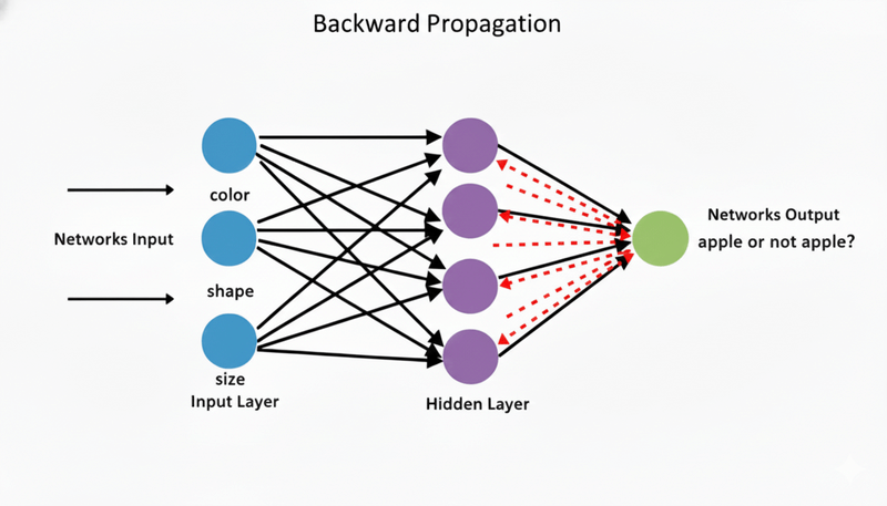
Output Layer (1 neuron) → adjust its weights ↓ Hidden Layer (4 neurons) → adjust its weights ↓ Input Layer (3 neurons)

That's why it's called "backward propagation" - we propagate (spread) the error information backward through the network, adjusting weights layer by layer.

Repeat Many Times Until It Learns

One iteration doesn't teach the network anything. Here's what happens:

Iteration 1:

• Forward Propagation: Make a prediction (probably wrong)
• Backward Propagation: Adjust weights slightly
• New weights saved

Iteration 2:

• Forward Propagation: Make another prediction (slightly better)
• Backward Propagation: Adjust weights again
• New weights saved

Iteration 3, 4, 5... 1000:

• Repeat the same process
• Each time, the weights get better
• The predictions get more accurate
• The error gets smaller

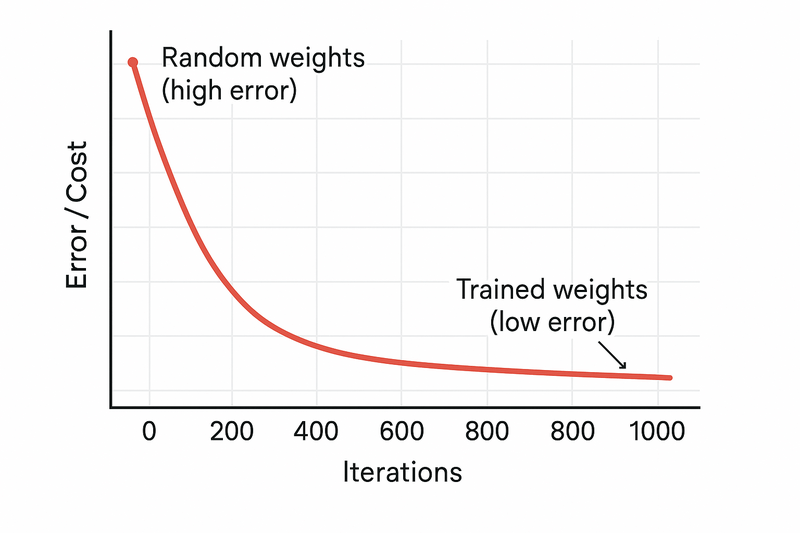
After 1000 iterations:

• The network has learned what weights work
• Now when you show it a new apple, it correctly predicts "yes, this is an apple"
• The cost function is low (error is small)
• We say the model is "trained"

The Complete Picture

Let me summarize what we covered:

1. Forward Propagation: Data flows from input → hidden layers → output. We make a prediction.

2. Measure Error: We compare prediction to actual answer using a cost function.

3. Backward Propagation: We calculate which weights caused the error and adjust them slightly in the right direction.

4. Repeat: We do this thousands of times until the error is very small and the network learned useful weights.

This is the entire learning process. Nothing magical. Just:

• Make a guess
• See if you were wrong
• Adjust your thinking slightly
• Repeat

Your brain does this when you learn. A baby learns an apple by seeing it many times, noticing when they're wrong, and adjusting their understanding. Neural networks do the same thing.

What's Next?

We've now covered:

• Issue #34: What are neural networks?
• Issue #35: How do neurons, weights, and biases work?
• Issue #36: How do networks learn (forward + backward propagation)?

Next week, we'll talk about something we mentioned but didn't explain deeply: Activation Functions. These are the functions that turn neuron outputs into 0-1 range (remember the "Final Output = Activation Function(Output)" part?). Why do we need them? What do they do? What are the different types? That's for next week.

📰 This Week in AI