Training Neural Networks: The Complete Learning Loop

Hey folks,

Last week we covered gradient descent - how neural networks use gradients to update weights and minimize loss.

This week: How do all these pieces actually come together to train a model?

We know how neural networks make predictions, calculate loss, find responsible weights, and update them. But what does the complete training process look like from start to finish?

Let's break it down.

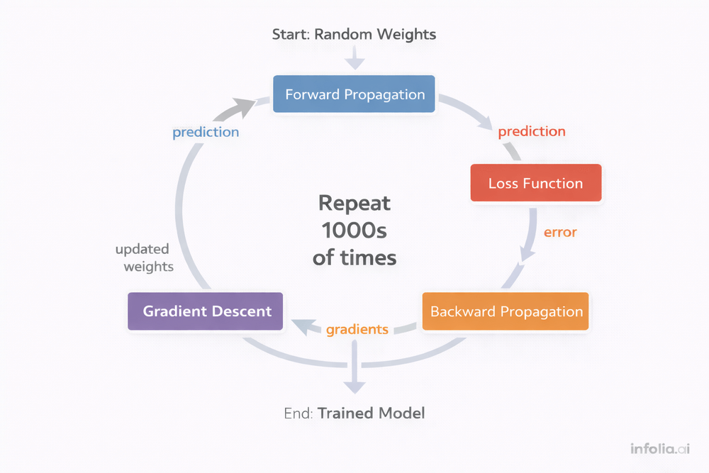
The Complete Training Loop

Training a neural network is an iterative cycle that repeats thousands of times until the model learns.

The loop works like this:

1. Initialize weights with random values
2. Forward propagation → make prediction
3. Calculate loss → measure error
4. Backward propagation → find responsible weights
5. Gradient descent → update weights
6. Repeat steps 2-5 many times
7. Stop when model performance plateaus

Each component you've learned fits into this cycle.

How Training Actually Works

Training begins with random weights. The network knows nothing about the problem. For a 10-class classification problem like digit recognition, initial accuracy is around 10% - equivalent to random guessing.

Example: Training an image classifier on 1000 images (500 cats, 500 dogs)

Iteration 1:

Random weights (network knows nothing)
Forward prop → prediction: "cat" (wrong, it's a dog)
Loss: 2.5 (very high error)
Backward prop → calculate gradients
Gradient descent → make tiny weight adjustments

Iteration 10:

Slightly improved weights
Prediction: still mostly wrong
Loss: 1.8 (lower than before)

Iteration 100:

Weights learning actual patterns
Prediction: correct 60% of the time
Loss: 0.4 (significantly better)

Iteration 1000:

Well-tuned weights
Prediction: correct 95% of the time
Loss: 0.1 (excellent performance)

Each iteration follows the same cycle: forward propagation → loss calculation → backward propagation → gradient descent weight update. The model improves incrementally with each pass.

This is the power of iterative learning. Small improvements compound over thousands of iterations.

Key Training Concepts

Epochs

An epoch represents one complete pass through the entire training dataset.

For a dataset with 60,000 training images:

• 1 epoch = network processes all 60,000 images once
• 10 epochs = network processes all 60,000 images ten times

Why multiple epochs? The network needs repeated exposure to examples. First pass, it learns basic features like edges and colors. Second pass, it refines understanding of shapes. By the tenth pass, complex patterns are well-established.

Typical training runs for 20-100 epochs depending on dataset size and problem complexity.

Batches and Why They Matter

Training divides data into batches rather than processing everything simultaneously.

Example:

• Dataset: 60,000 images
• Batch size: 32
• Batches per epoch: 1,875

Why use batches?

Memory efficiency: GPU can't hold 60,000 images at once. Batches of 32 fit easily.

Update frequency: Batch size 32 means 1,875 weight updates per epoch instead of one. More updates = faster learning.

Generalization: Batch variation helps the model learn robust patterns instead of memorizing.

Practical impact: Too small (size 1) = noisy, slow training. Too large (size 10,000) = fewer updates, memory issues. Sweet spot: 32-128.

Common batch sizes: 16, 32, 64, 128, 256

Iterations

An iteration is processing one batch.

1 epoch = 1,875 iterations (for batch size 32)
1 iteration = 32 images processed

For 10 epochs with 60,000 images: 18,750 total weight updates.

Training, Validation, and Test Data

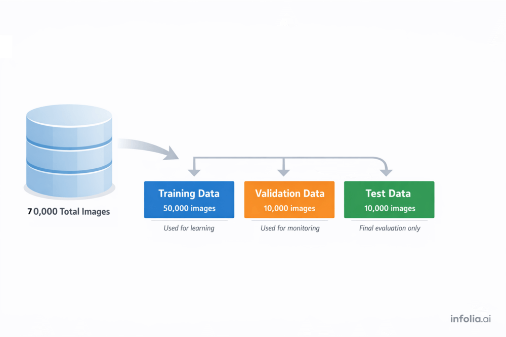
Data splits three ways:

Training data (50,000 images): Where learning happens. The network adjusts weights based on these examples.

Validation data (10,000 images): Monitoring system. After each epoch, check validation loss. If it stops improving, stop training. This is early stopping.

Why validation matters: Training loss almost always decreases with more training. But that doesn't mean improvement - the model might be memorizing. Validation loss reveals if the model is learning generalizable patterns.

Test data (10,000 images): Final exam. Use exactly once at the end to measure true performance on unseen data.

Common mistake: Using test data during training or making decisions based on test performance. This inflates metrics artificially.

Overfitting vs Underfitting

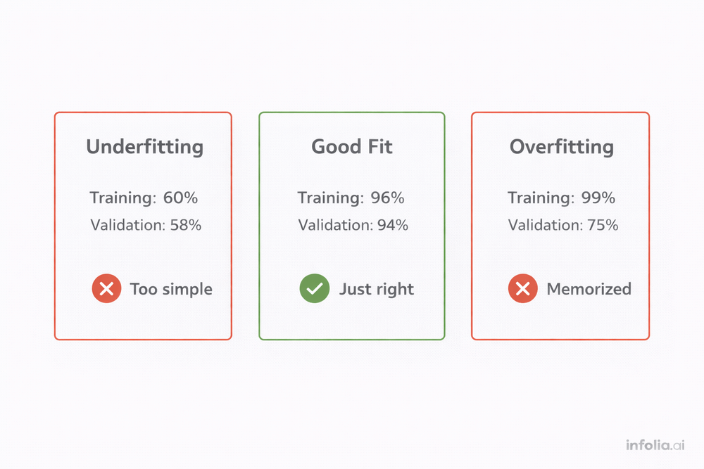
Underfitting

Training: 60%
Validation: 58%

Both metrics are low. The model hasn't learned enough.

Why this happens: Not enough training, model too simple, or learning rate too low.

Solutions: Train longer, add layers/neurons, increase learning rate.

Overfitting

Training: 99%
Validation: 75%

Classic overfitting signature. Great training, poor validation.

What's happening: The model memorized training examples instead of learning patterns. Like memorizing practice test questions without understanding concepts - perfect practice score, fails the real exam.

Warning sign: Training accuracy improves while validation accuracy plateaus or degrades.

Solutions: Stop training earlier (early stopping), use dropout (randomly disable neurons during training), get more data, reduce model complexity, or add regularization.

Optimal Fit

Training: 96%
Validation: 94%

Close performance on both datasets (2-3% gap). The model learned generalizable patterns. This is the goal.

Common Training Problems

Loss Not Decreasing

Symptoms: Loss stays constant across many epochs.

Epoch 1: Loss = 2.3
Epoch 50: Loss = 2.3

Possible causes: Learning rate too low, poor weight initialization, data not normalized, wrong loss function.

Solutions: Increase learning rate (0.0001 → 0.001), normalize inputs to [0,1], verify loss function matches problem type.

Loss Exploding

Symptoms: Loss shoots up to NaN.

Epoch 1: Loss = 2.3
Epoch 3: Loss = NaN

Why: Learning rate too high. Algorithm overshoots and hits numerical instability.

Solutions: Reduce learning rate (0.1 → 0.01), implement gradient clipping, use batch normalization.

Training Too Slow

Symptoms: One epoch takes 30+ minutes.

Causes: Batch size too small, using CPU instead of GPU, model too large.

Solutions: Increase batch size (32 → 128), switch to GPU (10-100x speedup), simplify architecture.

Critical Hyperparameters

Learning Rate: Weight update magnitude. Too high: explodes. Too low: never converges. Start: 0.001.

Batch Size: Examples per update. Larger: faster, more memory. Smaller: slower, less memory. Start: 32-64.

Epochs: Complete data passes. Too few: underfitting. Too many: overfitting. Start: 20-50, use early stopping.

How Everything Connects

Over the past seven weeks, you've learned individual components. Here's how they work together:

Foundation (Issues #34-35): Neural networks are layers of neurons with weights and biases.

Data Flow (Issue #36): Forward propagation generates predictions. Backward propagation calculates gradients.

Learning Mechanisms (Issues #37-39): Activation functions introduce non-linearity. Loss functions measure errors. Gradient descent optimizes weights.

The Complete Loop (Issue #40): All components work together in an iterative cycle.

Initialize Random Weights
         ↓
[Forward Prop → Loss → Backward Prop → Gradient Descent]
         ↓
    Repeat 1000s of times
         ↓
    Trained Model

Each iteration makes tiny improvements. After 10,000 iterations, random weights become a model that recognizes faces, translates languages, or generates images.

Key Takeaway

Training a neural network is fundamentally an iterative optimization process.

The cycle repeats thousands of times:

1. Generate predictions using forward propagation
2. Measure errors with the loss function
3. Find responsible weights via backward propagation
4. Adjust weights using gradient descent

Each iteration produces small improvements. After thousands of iterations, random weights transform into a trained model.

The key insight: The magic isn't in any individual step. It's in the repetitive cycle.

Run this loop 10,000 times, and random weights become a model that can recognize handwriting, understand speech, or generate realistic images.

The complete picture: You started with individual concepts - neurons, weights, activation functions, loss functions, gradients. Now you see how they work together in practice. This is the foundation that powers everything in modern AI, from ChatGPT to image generators to recommendation systems.

What's Next

Next week: Tensors and modern architectures.

Read the full AI Learning series → Learn AI