How Neural Networks Actually Learn (Gradient Descent)

Hey folks,

Last week we covered loss functions - how neural networks measure their mistakes.

This week: How do we use that measurement to improve the model?

We know the loss. Backward propagation tells us which weights caused it and by how much. But how do we actually adjust those weights to reduce the loss?

Let's break it down.

The Problem

Neural networks have thousands, sometimes millions of weights. Each weight affects the final loss.

The challenge: adjusting all these weights to minimize loss requires a systematic approach. That's what gradient descent provides.

What Gradient Descent Actually Is

Gradient descent is an optimization algorithm that adjusts weights to minimize loss.

The algorithm works by:

• Calculating the slope (called a "gradient") for each weight, showing which direction increases or decreases loss
• Taking small steps in the direction that reduces loss
• Repeating until loss stops decreasing

Consider this analogy: A hiker trying to reach the lowest valley in a mountain range while surrounded by thick fog. Unable to see the whole landscape, the hiker feels the slope beneath their feet and walks downhill, one step at a time, until reaching the valley.

Gradient descent follows the same principle.

The Mountain Analogy

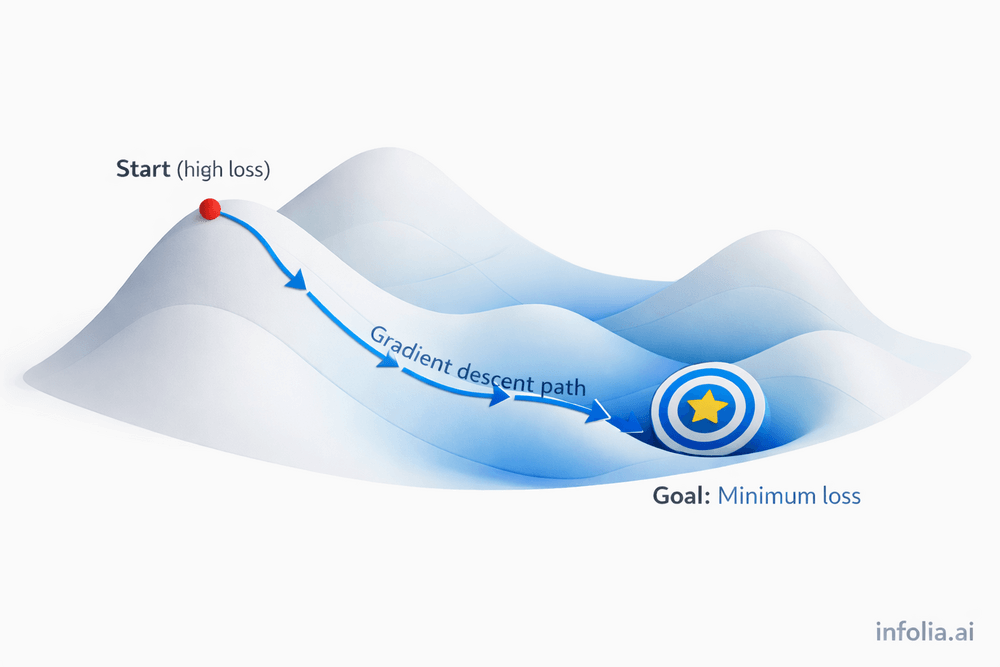
The loss function can be visualized as a mountain landscape where the current position represents current weights and their loss. The goal is finding the lowest valley (minimum loss).

The strategy: determine the slope at the current position and move downhill. Continue until reaching a valley. This is how gradient descent adjusts weights.

How It Actually Works

The gradient descent process follows these steps:

Step 1: Start with random weights

The network initializes with random weights. Initial loss is typically high.

Step 2: Calculate the loss

Forward propagation generates a prediction. The loss function (from Issue #38) compares it to the actual answer and calculates the loss.

Step 3: Calculate gradients

Backward propagation (covered in Issue #36) calculates how much each weight contributed to the loss. This calculation produces a "gradient" for each weight, essentially the slope that tells us: if we increase this weight, does the loss go up or down, and by how much?

Step 4: Update the weights

The key formula:

new_weight = old_weight - (learning_rate × gradient)

Each weight moves in the opposite direction of its gradient. Why opposite? The gradient points toward higher loss. We want to go the opposite way, toward lower loss.

Step 5: Repeat

Forward propagation runs again with updated weights. Loss is recalculated. Gradients are recomputed. Weights are updated again.

This cycle continues until the loss stops decreasing significantly.

The Learning Rate

The learning rate in the update formula controls the step size:

new_weight = old_weight - (learning_rate × gradient)

If the learning rate is too high:

Large steps cause overshooting. The algorithm bounces around the minimum without converging. Loss may increase instead of decrease.

If the learning rate is too low:

Tiny steps result in extremely slow training. Progress occurs but requires many iterations.

Finding the right learning rate is essential for efficient training. Common values include 0.001, 0.01, and 0.1. Experimentation is often needed to find the optimal value for a specific problem.

Three Types of Gradient Descent

There are three main variations, based on how much data you use per update.

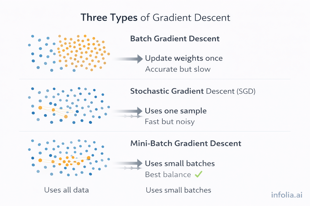
1. Batch Gradient Descent

Uses the entire dataset for each weight update.

Calculate loss across all samples, then update weights once. Accurate but slow, especially for large datasets. Best for small datasets (thousands of samples).

2. Stochastic Gradient Descent (SGD)

Uses one sample at a time.

Pick a random sample, calculate loss, update weights immediately. Fast but noisy. The loss bounces around but generally trends downward. Good for very large datasets (millions of samples).

3. Mini-Batch Gradient Descent

Uses small batches of data (typically 32, 64, or 128 samples).

Calculates average loss for the batch, then updates weights. Combines the accuracy of batch with the speed of SGD. Works efficiently with modern GPUs.

In practice: Mini-batch is the default choice. It balances speed and stability, making it ideal for most applications.

Common Problems

Problem 1: Learning Rate Too High

Symptoms: Loss increases or bounces erratically. The algorithm overshoots the minimum repeatedly.

Solution: Lower the learning rate. Try 0.01 instead of 0.1, or 0.001 instead of 0.01.

Problem 2: Learning Rate Too Low

Symptoms: Loss decreases extremely slowly. Training takes excessively long despite making progress.

Solution: Increase the learning rate. Try 0.01 instead of 0.001, or 0.1 instead of 0.01.

Problem 3: Local Minima

What it means: The algorithm reaches a valley, but not the lowest one.

Reality: This was a major concern historically, but modern deep networks with millions of parameters rarely encounter this issue. High-dimensional spaces don't have the same "local minima" problems as 2D landscapes.

Solutions if needed: Momentum (helps push through small hills), adaptive learning rates, or random restarts with different initial weights.

Practical Example

Training an image classifier on 1000 images (500 cats, 500 dogs):

Start: Random weights, loss = 2.5

After 10 iterations: Weights adjusted 10 times, loss = 1.8

After 100 iterations: Network learning patterns, loss = 0.4

After 1000 iterations: Weights well-tuned, loss = 0.1

Each iteration follows the same cycle: forward propagation → loss calculation → backward propagation → gradient descent weight update. Repeated 1000 times, the network learns to classify accurately.

Why It's Called "Gradient Descent"

Gradient refers to the slope or direction of steepest increase. In neural networks, the gradient indicates which direction increases the loss.

Descent means going downhill.

The algorithm moves in the opposite direction of the gradient, which is downhill toward lower loss. Hence: Gradient Descent.

How Everything Connects

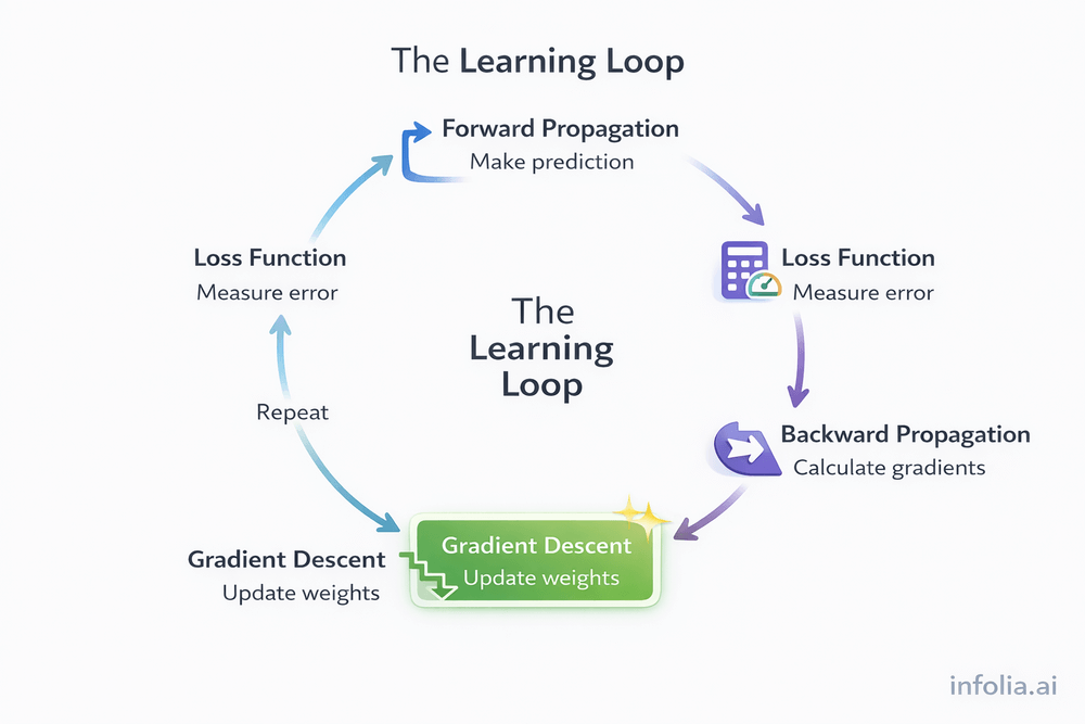
The complete learning loop:

1. Forward Propagation - Input → neurons → activation functions → prediction

2. Loss Function - Compare prediction to actual answer, calculate loss

3. Backward Propagation - Calculate how much each weight contributed to the loss

4. Gradient Descent - Use those gradients to update weights in the direction that reduces loss

5. Repeat - Run forward propagation again with new weights

This cycle continues until the loss converges. Gradient descent is what makes the learning loop functional.

Key Takeaway

Gradient descent is the optimization algorithm that enables neural network learning.

The process:

• Calculate the loss
• Calculate gradients via backward propagation
• Update weights in the opposite direction of the gradient
• Repeat until loss converges

The three types:

• Batch (entire dataset, accurate but slow)
• Stochastic (one sample, fast but noisy)
• Mini-batch (small batches, optimal balance)

The critical parameter:

• Learning rate (controls step size)

The mountain analogy captures the essence: moving downhill step by step, guided by the local slope, until reaching the lowest point. This is how neural networks learn.

What's Next

The complete learning process is now clear.

From neurons to weights, forward propagation to activation functions, loss functions to backward propagation, and finally gradient descent.

The full cycle:

Input → Forward → Activation → Prediction → Loss → Backward → Gradients → Gradient Descent → Updated Weights → Repeat

This foundation supports everything in deep learning.

Future topics will explore how to make this process faster, more stable, and more powerful.

Read the full AI Learning series:

1. What Neural Networks Actually Are
2. Neurons, Weights, Biases
3. Forward & Backward Propagation
4. Activation Functions
5. Loss Functions
6. Gradient Descent ← You are here

📰 This Week in AI