Convolutional Neural Networks: How AI Sees Images

Hey folks,

Last week we covered tensors - the multi-dimensional data structures that organize images as 4D arrays for batch processing.

This week: How neural networks actually process those image tensors.

Fully-connected networks from Issues #34-40 work for simple inputs. For images, we need something fundamentally different: Convolutional Neural Networks.

Let's break it down.

The Problem with Fully-Connected Networks

Standard neural networks connect every input to every neuron in the first layer.

For a 224×224 color image:

Input size: 224 × 224 × 3 = 150,528 pixels
First hidden layer: 1,000 neurons
Parameters needed: 150,528 × 1,000 = 150,528,000

150 million parameters for just the first layer.

Three critical problems:

1. Too many parameters
Models become massive. Training requires enormous computational resources and vast amounts of data to avoid overfitting.

2. Spatial relationships ignored
Flattening a 224×224 image into a 150,528-element vector destroys spatial structure. The network doesn't know that pixel (100, 50) is near pixel (100, 51). Nearby pixels—which typically form edges, textures, and objects—are treated as independent.

3. Position-dependent learning
A cat in the top-left corner requires different learned weights than a cat in the bottom-right corner. The network must learn to recognize cats separately in every possible position.

Images have spatial structure. Fully-connected networks don't exploit it.

CNNs solve this.

What Convolution Actually Is

Convolution is a mathematical operation that slides a small filter across an image, computing local patterns.

The process:

1. Take a small filter (typically 3×3 or 5×5)
2. Place it at the top-left corner of the image
3. Compute the dot product (element-wise multiplication, then sum)
4. Slide the filter one pixel to the right
5. Repeat across the entire image

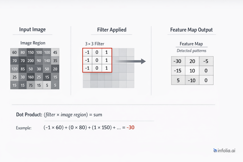
Simple example: 3×3 edge detection filter

Filter (detects vertical edges):
[[-1,  0,  1],
 [-1,  0,  1],
 [-1,  0,  1]]

Image region:
[[100, 100, 50],
 [100, 100, 50],
 [100, 100, 50]]

Convolution result:
(-1×100) + (0×100) + (1×50) +
(-1×100) + (0×100) + (1×50) +
(-1×100) + (0×100) + (1×50) = -150

Strong negative response indicates vertical edge detected

The same filter slides across every position in the image, detecting the same pattern everywhere.

Filters and Feature Detection

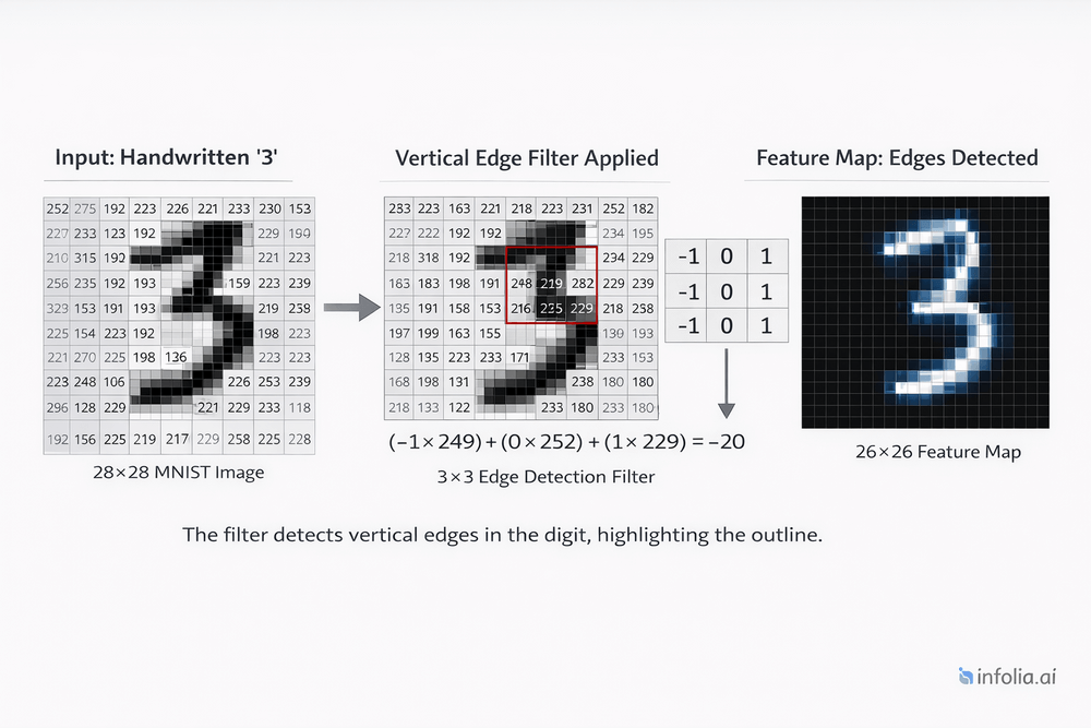
Filters (also called kernels) detect specific patterns. Neural networks learn these filters during training.

What different layers detect:

Early layers (Layer 1-2):

• Horizontal edges
• Vertical edges
• Diagonal edges
• Color gradients
• Simple corners

Middle layers (Layer 3-5):

• Textures (stripes, dots, grids)
• Simple shapes (circles, rectangles)
• Color patterns
• Repeated motifs

Deep layers (Layer 6+):

• Complex objects (eyes, wheels, windows)
• Faces
• Animal parts
• Object components

Critical insight: These filters are not manually designed. The network learns them automatically through backpropagation, discovering which patterns are most useful for the task.

Feature Maps

Applying one filter to an image produces one feature map.

Example:

Input: 224×224×3 color image
Filter: 3×3 edge detector
Output: 222×222 feature map (slightly smaller due to filter size)

CNNs use many filters simultaneously:

Input: 224×224×3
Apply 32 different 3×3 filters
Output: 222×222×32 (32 feature maps)

Each of the 32 filters detects a different pattern. The output is a 3D tensor where each "slice" represents one detected feature across the entire image.

Shape transformation:

(224, 224, 3) → [Conv with 32 filters] → (222, 222, 32)

More filters = more patterns detected = richer representation.

Pooling Layers

Pooling reduces spatial dimensions while retaining important information.

Max pooling (most common):

1. Divide the feature map into regions (typically 2×2)
2. Take the maximum value from each region
3. Output a smaller feature map

Example:

Input region (2×2):
[[8,  3],
 [4,  2]]

Max pool output: 8 (maximum value)

Effect on dimensions:

Input: 222×222×32
Max pooling (2×2)
Output: 111×111×32

Height and width reduced by half. Number of channels (32) unchanged.

Why pooling matters:

Dimensionality reduction: Fewer parameters in subsequent layers, faster computation.

Translation invariance: Small shifts in object position don't change the pooled output. A cat moved 1 pixel still produces the same max pooled features.

Focus on presence, not position: Max pooling asks "Is this feature present in this region?" rather than "Exactly where is it?"

CNN Architecture

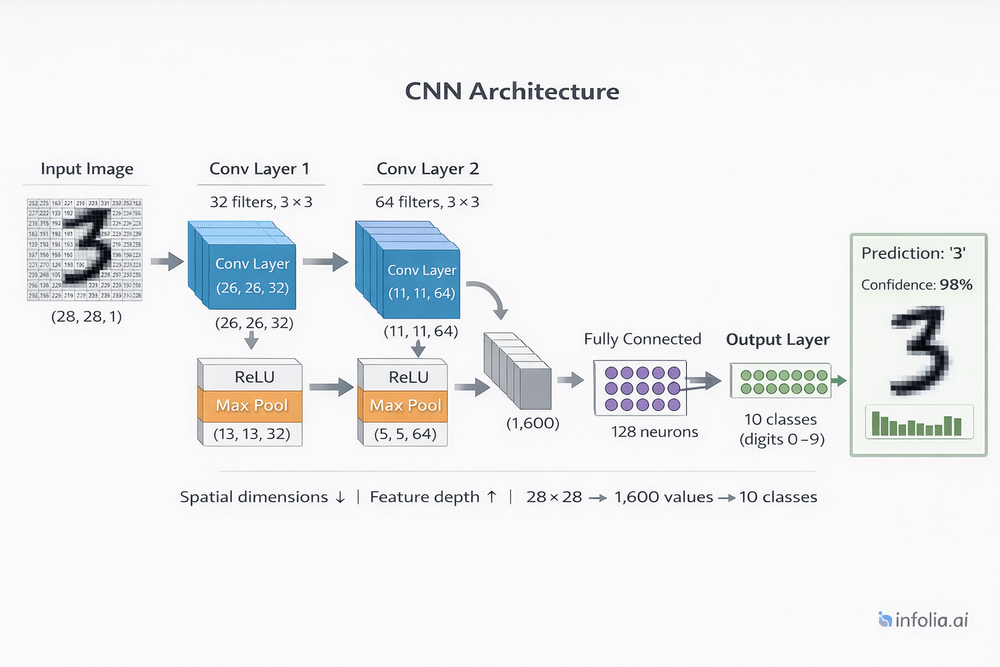
Modern CNNs stack multiple convolutional and pooling layers.

Typical structure:

Input Image (224×224×3)
    ↓
[Conv Layer] → 32 filters, 3×3 → (222×222×32)
[ReLU Activation]
[Max Pool] → 2×2 → (111×111×32)
    ↓
[Conv Layer] → 64 filters, 3×3 → (109×109×64)
[ReLU Activation]
[Max Pool] → 2×2 → (54×54×64)
    ↓
[Conv Layer] → 128 filters, 3×3 → (52×52×128)
[ReLU Activation]
[Max Pool] → 2×2 → (26×26×128)
    ↓
[Flatten] → (26×26×128 = 86,528)
    ↓
[Fully Connected] → 1,000 neurons
[ReLU Activation]
    ↓
[Fully Connected] → 10 classes (output)
[Softmax Activation]
    ↓
Class Predictions

Pattern: As depth increases, spatial dimensions decrease (224→111→54→26) while channels increase (3→32→64→128).

Early layers capture simple features across large spatial areas. Deep layers capture complex features in smaller, more abstract spaces.

Why CNNs Work for Images

Three key principles make CNNs effective:

Parameter Sharing

The same filter applies to every position in the image.

Fully-connected approach:

• Different weights for cat detection at position (50, 50) vs (100, 100)
• Must learn "cat" separately for every location
• Millions of redundant parameters

CNN approach:

• Single cat-detection filter slides across entire image
• Same weights everywhere
• Learn once, apply everywhere

A 3×3 filter has 9 parameters. These 9 parameters apply to every position, not 9 parameters per position.

Spatial Locality

Images have local structure. Nearby pixels are related—they form edges, textures, and objects.

CNNs exploit this by:

• Processing small local regions (3×3, 5×5)
• Building complex features hierarchically
• Preserving spatial relationships through convolution

A pixel at (100, 50) is processed with its neighbors (100, 51), (101, 50), etc. Their relationships are preserved.

Translation Invariance

Objects can appear anywhere in an image. CNNs detect them regardless of position.

A vertical edge filter detects vertical edges in the top-left, center, and bottom-right equally well. The same learned filter slides across all positions.

This is why CNNs work for object detection: a cat is recognized whether it's in the corner or the center.

Image Classification Pipeline

Complete flow through a CNN for image classification:

Input:

Batch of 32 color images
Shape: (32, 224, 224, 3)

Convolutional layers:

Layer 1: (32, 222, 222, 32)   # 32 filters detect edges
Layer 2: (32, 109, 109, 64)   # 64 filters detect textures
Layer 3: (32, 52, 52, 128)    # 128 filters detect patterns

Spatial dimensions shrink (224→222→109→52). Feature depth grows (3→32→64→128).

Flatten:

(32, 52, 52, 128) → (32, 346,112)

Convert 3D feature maps to 1D vectors.

Fully-connected layers:

(32, 346,112) → (32, 1,000) → (32, 10)

Standard neural network layers make final classification decisions.

Output:

(32, 10)
32 images, 10 class probabilities each

Softmax activation converts final layer outputs to probabilities that sum to 1.0 per image.

Real-World CNN Examples

LeNet-5 (1998):
First successful CNN for handwritten digit recognition (MNIST).
Structure: 2 conv layers, 2 pooling layers, 3 FC layers.
Achievement: 99%+ accuracy on digit classification.

AlexNet (2012):
Breakthrough that revived deep learning.
Structure: 5 conv layers, 3 FC layers, 60M parameters.
Achievement: Won ImageNet competition, reduced error rate by 10%.

VGG-16 (2014):
Very deep network with small 3×3 filters throughout.
Structure: 13 conv layers, 3 FC layers, 138M parameters.
Achievement: Showed deeper networks with smaller filters outperform shallow networks with large filters.

ResNet (2015):
Introduced skip connections, enabling training of 50-152 layer networks.
Achievement: Won ImageNet with 3.6% error (better than human performance at 5%).

All modern computer vision—object detection, face recognition, medical imaging—builds on these CNN principles.

Key Takeaway

Convolutional Neural Networks exploit spatial structure in images through three core principles:

Parameter sharing: Same filter applies everywhere, dramatically reducing parameters.

Spatial locality: Process local regions, preserve relationships between nearby pixels.

Translation invariance: Detect patterns regardless of position in the image.

The architecture: Stack conv layers (detect features) and pooling layers (reduce dimensions) to build hierarchical representations. Early layers detect simple patterns. Deep layers combine them into complex object representations.

CNNs transform the computer vision problem from "learn every pixel independently" to "learn reusable spatial filters that compose hierarchically."

This is why CNNs power facial recognition, medical imaging, autonomous vehicles, and visual search.

What's Next

Next week: Recurrent Neural Networks (RNNs) and processing sequential data.

Read the full AI Learning series → Learn AI